16S Metagenomics Training - Chaillou dataset analysis

Introduction
This vignette is a re-analysis of the data set from Chaillou et al. (2015), as suggested in the Homeworks section of the slides. Note that this is only one of many analyses that could be done on the data.
Analysis
Setup
We first setup our environment by loading a few packages
library(tidyverse)  ## data manipulation
library(phyloseq)   ## analysis of microbiome census data
library(ape)        ## for tree manipulation
library(vegan)      ## for community ecology analyses
library(phyloseq.extended)
library(scales)
## You may also need to install gridExtra with
## install.packages("gridExtra")
## and load it with
## library(gridExtra)
## if you want to reproduce some of the side-by-side graphs shown below
Data import
We then load the data from the Chaillou et al. (2015) dataset. We assume that they are located in the data/chaillou folder. A quick look at the folder content shows we have access to a tree (in newick format, file extension nwk) and a biom file (extension biom). A glance at the biom file content shows that the taxonomy is "k__Bacteria", "p__Tenericutes", "c__Mollicutes", "o__Mycoplasmatales", "f__Mycoplasmataceae", "g__Candidatus Lumbricincola", "s__NA". This is the so called greengenes format and the taxonomy should thus be parsed using the parse_taxonomy_greengenes function.
food <- import_biom("chaillou_data/chaillou.biom",
                    parseFunction = parse_taxonomy_greengenes)
metadata <- read.table("chaillou_data/chaillou_metadata.tsv", row.names=1, header=TRUE, sep="\t", stringsAsFactors = FALSE)
sample_data(food) <- metadata
We can then add the phylogenetic tree to the food object
phy_tree(food) <- read_tree("chaillou_data/tree.nwk")
food
## phyloseq-class experiment-level object
## otu_table() OTU Table: [ 508 taxa and 64 samples ]
## sample_data() Sample Data: [ 64 samples by 3 sample variables ]
## tax_table() Taxonomy Table: [ 508 taxa by 7 taxonomic ranks ]
## phy_tree() Phylogenetic Tree: [ 508 tips and 507 internal nodes ]The data consists of 64 samples of food: 8 replicates for each of 8 food types. We have access to the following descriptors
- EnvType: Food of origin of the samples
- FoodType: Either meat or seafood
- Description: Replicate number
We can navigate through the metadata
##                     EnvType Description FoodType
## DLT0.LOT08       DesLardons        LOT8     Meat
## DLT0.LOT05       DesLardons        LOT5     Meat
## DLT0.LOT03       DesLardons        LOT3     Meat
## DLT0.LOT07       DesLardons        LOT7     Meat
## DLT0.LOT06       DesLardons        LOT6     Meat
## DLT0.LOT01       DesLardons        LOT1     Meat
## DLT0.LOT04       DesLardons        LOT4     Meat
## DLT0.LOT10       DesLardons       LOT10     Meat
## MVT0.LOT05 SaucisseVolaille        LOT5     Meat
## MVT0.LOT01 SaucisseVolaille        LOT1     Meat
## MVT0.LOT06 SaucisseVolaille        LOT6     Meat
## MVT0.LOT07 SaucisseVolaille        LOT7     Meat
## MVT0.LOT03 SaucisseVolaille        LOT3     Meat
## MVT0.LOT09 SaucisseVolaille        LOT9     Meat
## MVT0.LOT08 SaucisseVolaille        LOT8     Meat
## MVT0.LOT10 SaucisseVolaille       LOT10     Meat
## BHT0.LOT01       BoeufHache        LOT1     Meat
## BHT0.LOT07       BoeufHache        LOT7     Meat
## BHT0.LOT06       BoeufHache        LOT6     Meat
## BHT0.LOT03       BoeufHache        LOT3     Meat
## BHT0.LOT10       BoeufHache       LOT10     Meat
## BHT0.LOT05       BoeufHache        LOT5     Meat
## BHT0.LOT04       BoeufHache        LOT4     Meat
## BHT0.LOT08       BoeufHache        LOT8     Meat
## VHT0.LOT02        VeauHache        LOT2     Meat
## VHT0.LOT10        VeauHache       LOT10     Meat
## VHT0.LOT03        VeauHache        LOT3     Meat
## VHT0.LOT01        VeauHache        LOT1     Meat
## VHT0.LOT08        VeauHache        LOT8     Meat
## VHT0.LOT06        VeauHache        LOT6     Meat
## VHT0.LOT07        VeauHache        LOT7     Meat
## VHT0.LOT04        VeauHache        LOT4     Meat
## SFT0.LOT08       SaumonFume        LOT8  Seafood
## SFT0.LOT07       SaumonFume        LOT7  Seafood
## SFT0.LOT06       SaumonFume        LOT6  Seafood
## SFT0.LOT03       SaumonFume        LOT3  Seafood
## SFT0.LOT02       SaumonFume        LOT2  Seafood
## SFT0.LOT05       SaumonFume        LOT5  Seafood
## SFT0.LOT04       SaumonFume        LOT4  Seafood
## SFT0.LOT01       SaumonFume        LOT1  Seafood
## FST0.LOT07      FiletSaumon        LOT7  Seafood
## FST0.LOT08      FiletSaumon        LOT8  Seafood
## FST0.LOT05      FiletSaumon        LOT5  Seafood
## FST0.LOT06      FiletSaumon        LOT6  Seafood
## FST0.LOT01      FiletSaumon        LOT1  Seafood
## FST0.LOT03      FiletSaumon        LOT3  Seafood
## FST0.LOT10      FiletSaumon       LOT10  Seafood
## FST0.LOT02      FiletSaumon        LOT2  Seafood
## FCT0.LOT06   FiletCabillaud        LOT6  Seafood
## FCT0.LOT10   FiletCabillaud       LOT10  Seafood
## FCT0.LOT05   FiletCabillaud        LOT5  Seafood
## FCT0.LOT03   FiletCabillaud        LOT3  Seafood
## FCT0.LOT08   FiletCabillaud        LOT8  Seafood
## FCT0.LOT02   FiletCabillaud        LOT2  Seafood
## FCT0.LOT07   FiletCabillaud        LOT7  Seafood
## FCT0.LOT01   FiletCabillaud        LOT1  Seafood
## CDT0.LOT10         Crevette       LOT10  Seafood
## CDT0.LOT08         Crevette        LOT8  Seafood
## CDT0.LOT05         Crevette        LOT5  Seafood
## CDT0.LOT04         Crevette        LOT4  Seafood
## CDT0.LOT06         Crevette        LOT6  Seafood
## CDT0.LOT09         Crevette        LOT9  Seafood
## CDT0.LOT07         Crevette        LOT7  Seafood
## CDT0.LOT02         Crevette        LOT2  Seafood
EnvType is coded in French and with categories in no meaningful order. We will translate them and order them to have food type corresponding to meat first and to seafood second.
## We create a "dictionary" for translation and order the categories
## as we want
dictionary = c("BoeufHache"      = "Ground_Beef",
               "VeauHache"       = "Ground_Veal",
               "MerguezVolaille" = "Poultry_Sausage",
               "DesLardons"      = "Bacon_Dice",
               "SaumonFume"      = "Smoked_Salmon",
               "FiletSaumon"     = "Salmon_Fillet",
               "FiletCabillaud"  = "Cod_Fillet",
               "Crevette"        = "Shrimp")
env_type <- sample_data(food)$EnvType
sample_data(food)$EnvType <- factor(dictionary[env_type], levels = dictionary)
We can also build a custom color palette to remind ourselves which samples correspond to meat and which to seafood.
my_palette <- c('#67001f','#b2182b','#d6604d','#f4a582',
                 '#92c5de','#4393c3','#2166ac','#053061')
names(my_palette) <- dictionary
Before moving on to elaborate statistics, we’ll look at the taxonomic composition of our samples ## Taxonomic Composition {.tabset}
To use the plot_composition function, we first need to source it:
download.file(url = "https://raw.githubusercontent.com/mahendra-mariadassou/phyloseq-extended/master/R/graphical_methods.R",
              destfile = "graphical_methods.R")
source("graphical_methods.R")
We then look at the community composition at the phylum level. In order to highlight the structure of the data, we split the samples according to their food of origin. We show several figures, corresponding to different taxonomic levels.
Phylum level
We can see right away that meat products are whereas Bacteroidetes and Proteobacteria are more abundant in seafood.
plot_composition(food, "Kingdom", "Bacteria", "Phylum", fill = "Phylum") +
  facet_grid(~EnvType, scales = "free_x", space = "free_x") +
  theme(axis.text.x = element_blank())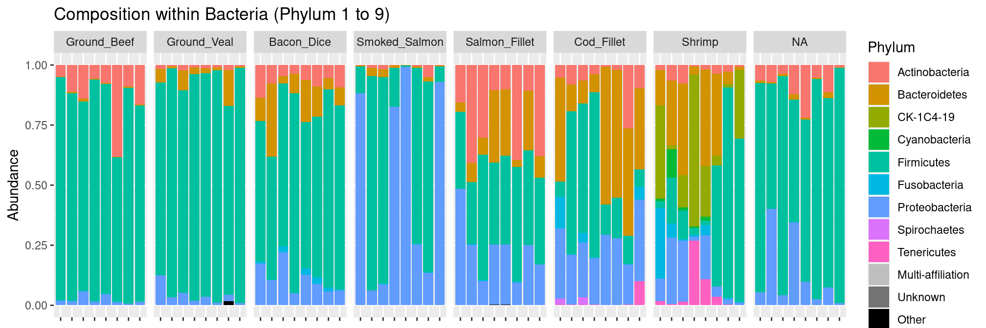
We have access to the following taxonomic ranks:
rank_names(food)## [1] "Kingdom" "Phylum" "Class" "Order" "Family" "Genus" "Species"Within firmicutes
Given the importance of Firmicutes, we can zoom in within that phylum and investigate the composition at the genus level.
plot_composition(food, "Phylum", "Firmicutes", "Genus", fill = "Genus", numberOfTaxa = 5) +
  facet_grid(~EnvType, scales = "free_x", space = "free_x") +
  theme(axis.text.x = element_blank())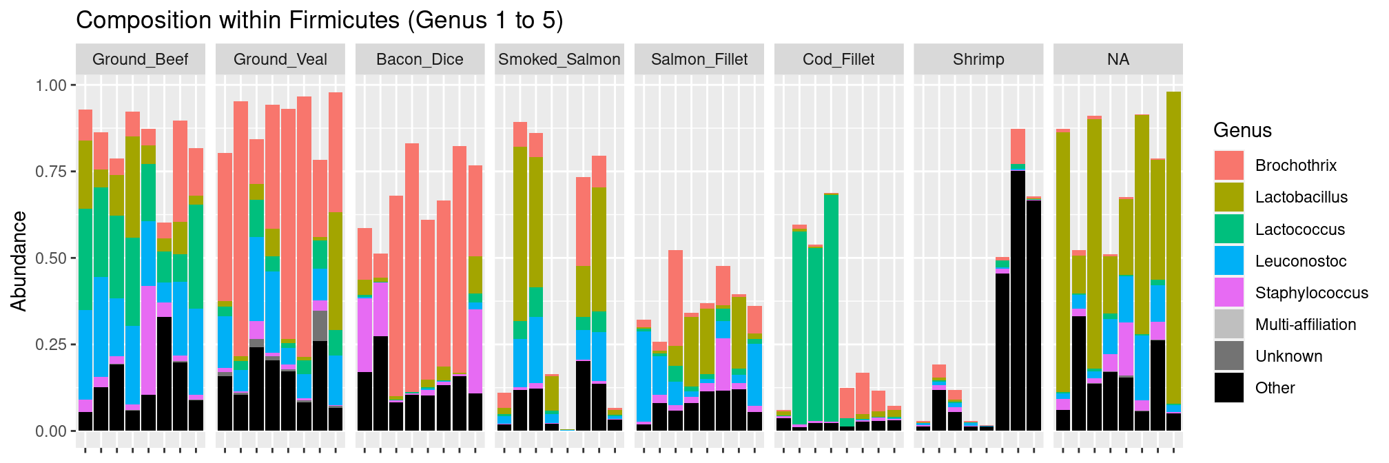
We see that there is a high diversity of genera across the different types of food and that no single OTU dominates all communities.
Alpha-diversity
The samples have very similar sampling depths
sample_sums(food) %>% range()## [1] 11718 11857there is thus no need for rarefaction.
Graphics
We compare the different types of food in terms of diversity.
plot_richness(food, x = "EnvType", color = "EnvType",
              measures = c("Observed", "Shannon", "InvSimpson")) +
  geom_boxplot(aes(group = EnvType)) +    ## add one boxplot per type of food
  scale_color_manual(values = my_palette) ## custom color palette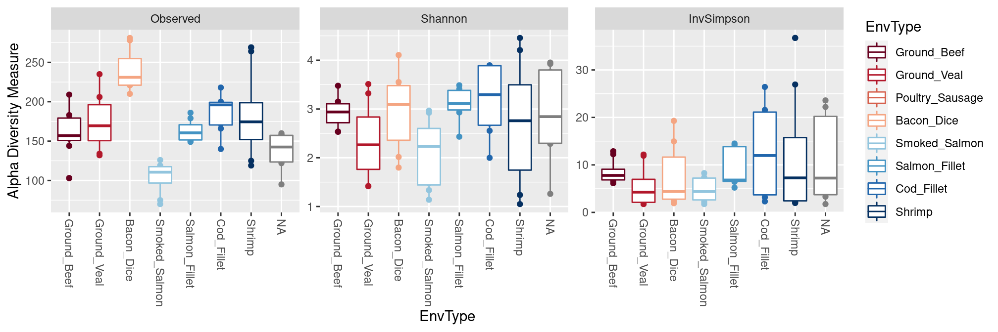
Different foods have very different diversities with dice of bacon having the highest number (\(\sim\) 250) of OTUs. However, most foods have low effective diversities.
Anova
We can quantify the previous claims by performing an ANOVA of the diversity against the covariates of interest. For the sake of brevity, we focus here on both the observed and effective number of species (as measured by the InvSimpson measure). We first build a data.frame with both covariates and diversity indices.
div_data <- cbind(estimate_richness(food),  ## diversity indices
                  sample_data(food)         ## covariates
                  )
Foods differ significantly in terms of number of observed OTUs…
model <- aov(Observed ~ EnvType, data = div_data)
anova(model)
## Analysis of Variance Table
##
## Response: Observed
## Df Sum Sq Mean Sq F value Pr(>F)
## EnvType 6 78171 13028.6 12.353 2.029e-08 ***
## Residuals 49 51680 1054.7
## ---
## Signif. codes: 0 '***' 0.001 '**' 0.01 '*' 0.05 '.' 0.1 ' ' 1… but no in terms of effective number of species
model <- aov(InvSimpson ~ EnvType, data = div_data)
anova(model)
## Analysis of Variance Table
##
## Response: InvSimpson
## Df Sum Sq Mean Sq F value Pr(>F)
## EnvType 6 444.63 74.105 1.4865 0.2025
## Residuals 49 2442.75 49.852Beta diversities
We have access to a phylogenetic tree so we can compute all 4 distances seen during the tutorial.
dist.jac <- distance(food, method = "cc")
dist.bc <- distance(food, method = "bray")
dist.uf <- distance(food, method = "unifrac")
dist.wuf <- distance(food, method = "wunifrac")
p.jac <- plot_ordination(food,
ordinate(food, method = "MDS", distance = dist.jac),
color = "EnvType") +
ggtitle("Jaccard") + scale_color_manual(values = my_palette)
p.bc <- plot_ordination(food,
ordinate(food, method = "MDS", distance = dist.bc),
color = "EnvType") +
ggtitle("Bary-Curtis") + scale_color_manual(values = my_palette)
p.uf <- plot_ordination(food,
ordinate(food, method = "MDS", distance = dist.uf),
color = "EnvType") +
ggtitle("UniFrac") + scale_color_manual(values = my_palette)
p.wuf <- plot_ordination(food,
ordinate(food, method = "MDS", distance = dist.wuf),
color = "EnvType") +
ggtitle("wUniFrac") + scale_color_manual(values = my_palette)
gridExtra::grid.arrange(p.jac, p.bc, p.uf, p.wuf,
ncol = 2)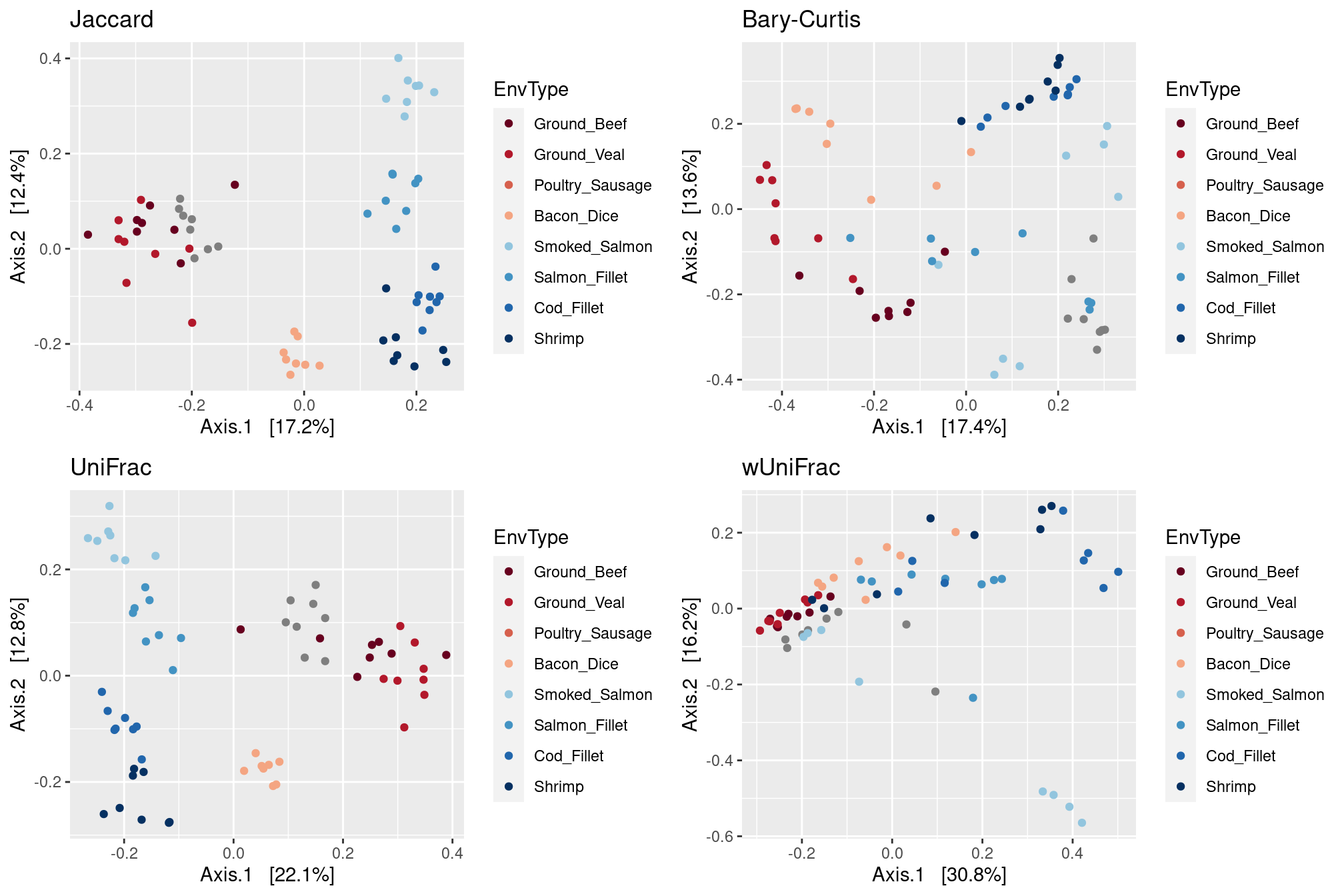
In this example, Jaccard and UniFrac distances provide a clear separation of meats and seafoods, unlike Bray-Curtis and wUniFrac. This means that food ecosystems share their abundant taxa but not the rare ones.
UniFrac also gives a much better separation of poultry sausages and ground beef / veal than Jaccard. This means that although those foods have taxa in common, their specific taxa are located in different parts of the phylogenetic tree. Since UniFrac appears to the most relevant distance here, we’ll restrict downstream analyses to it.
One can also note that dices of bacon are located between meats and seafoods. We’ll come back latter to that point latter.
Hierarchical clustering
The hierarchical clustering of uniFrac distances using the Ward linkage function (to produce spherical clusters) show a perfect separation according.
par(mar = c(1, 0, 2, 0))
plot_clust(food, dist = "unifrac", method = "ward.D2", color = "EnvType",
           palette = my_palette,
           title = "Clustering of samples (UniFrac + Ward)\nsamples colored by EnvType")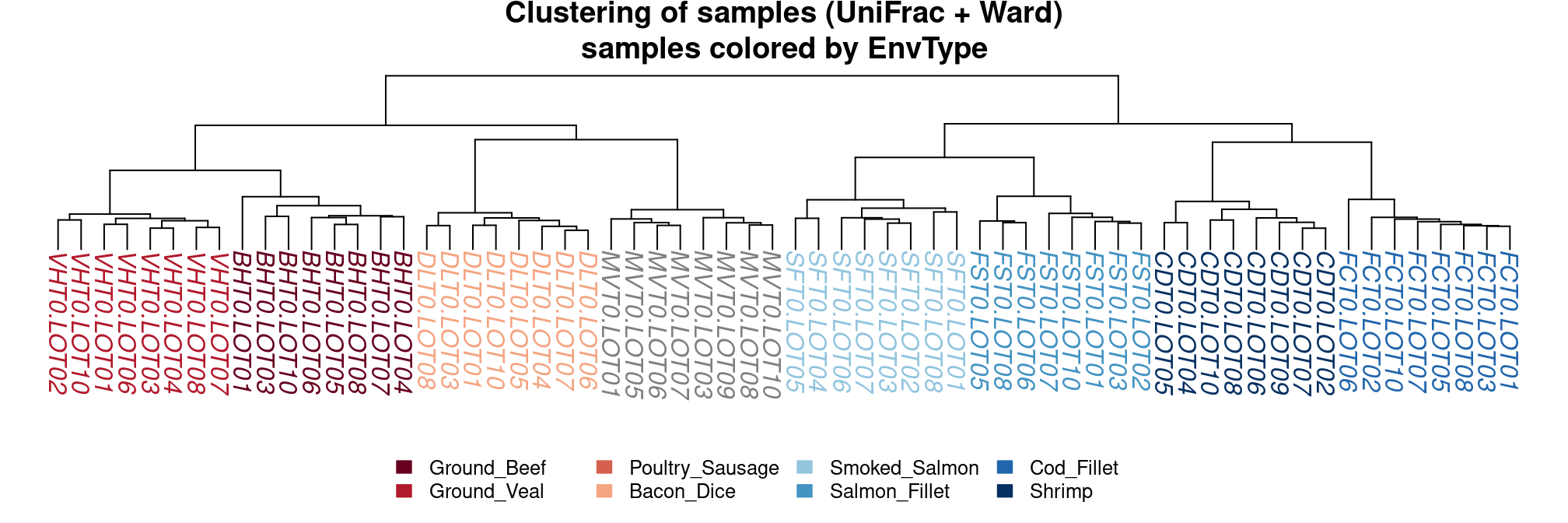
PERMANOVA
We use the Unifrac distance to assess the variability in terms of microbial repertoires between foods.
#metadata <- sample_data(food) %>% as("data.frame")
model <- adonis(dist.uf ~ EnvType, data = metadata, permutations = 999)
model
##
## Call:
## adonis(formula = dist.uf ~ EnvType, data = metadata, permutations = 999)
##
## Permutation: free
## Number of permutations: 999
##
## Terms added sequentially (first to last)
##
## Df SumsOfSqs MeanSqs F.Model R2 Pr(>F)
## EnvType 7 7.6565 1.09379 13.699 0.63132 0.001 ***
## Residuals 56 4.4713 0.07984 0.36868
## Total 63 12.1278 1.00000
## ---
## Signif. codes: 0 '***' 0.001 '**' 0.01 '*' 0.05 '.' 0.1 ' ' 1The results show that food origin explains a bit less than 2 thirds of the total variability observed between samples in terms of species repertoires. This is quite strong! Don’t expect such strong results in general.
Heatmap
We investigate the content of our samples when looking at the raw count table and use a custom color scale to reproduce (kind of) the figures in the paper.
p <- plot_heatmap(food) +
  facet_grid(~EnvType, scales = "free_x", space = "free_x") +
  scale_fill_gradient2(low = "#1a9850", mid = "#ffffbf", high = "#d73027",
                       na.value = "white", trans = log_trans(4),
                       midpoint = log(100, base = 4))
plot(p)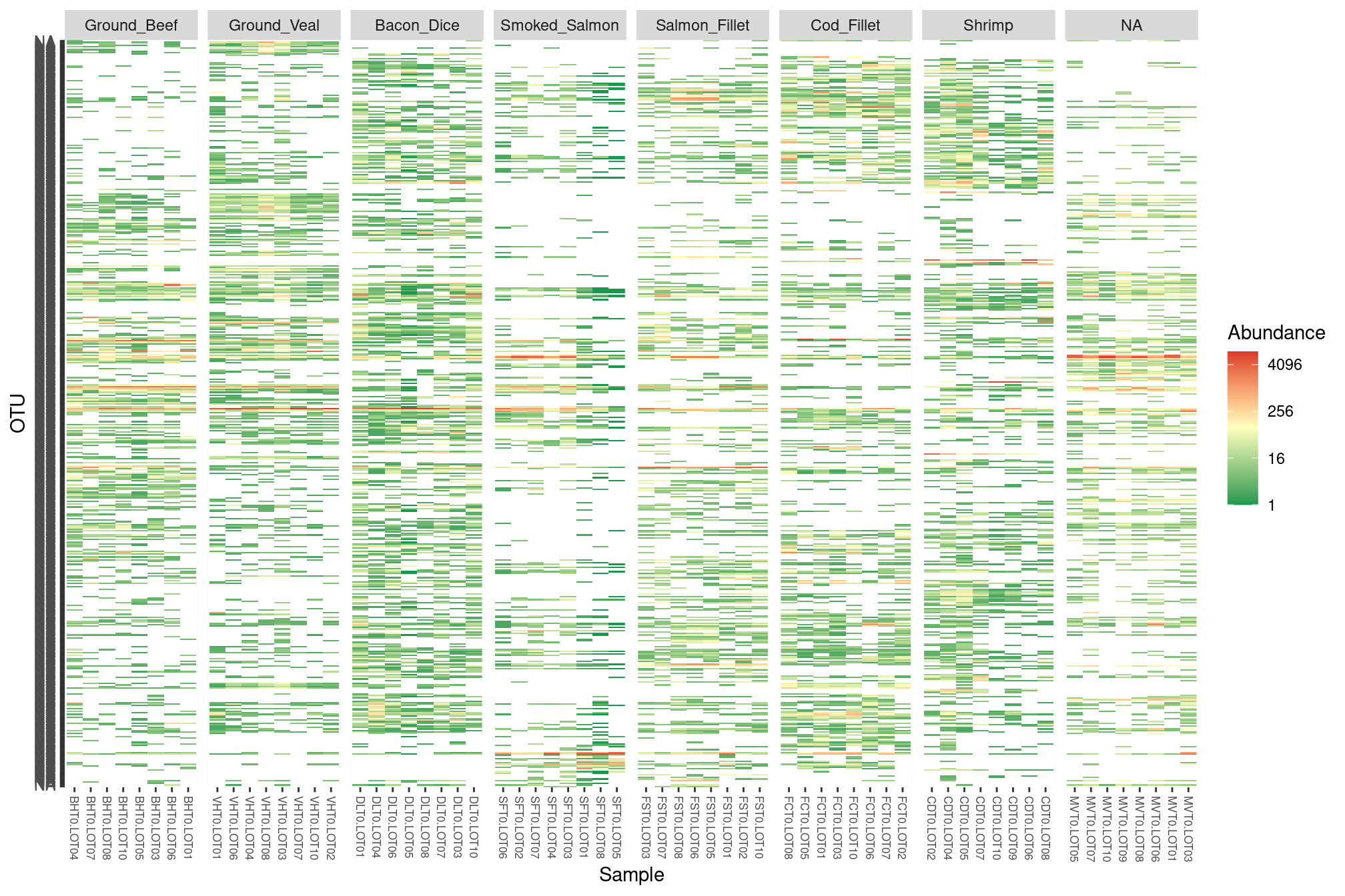
It looks like: - there is some kind of block structure in the data (eg. OTUs that are abundant in seafoods but not meat products or vice-versa) - dices of bacon have a lot of OTU in common with seafoods. This is indeed the case and the result of “contamination”, sea salt is usually added to bacon to add flavor. But, in addition to flavor, the grains of salt also bring sea-specific bacterial taxa (at least their genetic material) with them.
Differential abundance study
To highlight the structure, we’re going to perform a differential analysis (between meat products and seafoods) and look only at the differentially abundant taxa.
cds <- phyloseq_to_deseq2(food, ~ FoodType)
dds <- DESeq2::DESeq(cds)
results <- DESeq2::results(dds) %>% as.data.frame()
We can explore the full result table:
DT::datatable(results, filter = "top",
              extensions = 'Buttons',
              options = list(dom = "Bltip", buttons = c('csv'))) %>%
  DT::formatRound(columns = names(results), digits = 4)
Or only select the OTUs with an adjusted p-value lower than \(0.05\) and sort them according to fold-change.
da_otus <- results %>% as_tibble(rownames = "OTU") %>%
  filter(padj < 0.05) %>%
  arrange(log2FoldChange) %>%
  pull(OTU)
length(da_otus)
## [1] 273We end up with 273 significant OTUs sorted according to their fold-change. We keep only those OTUs in that order in the heat map.
p <- plot_heatmap(prune_taxa(da_otus, food), ## keep only da otus...
                  taxa.order = da_otus       ## ordered according to fold-change
                  ) +
  facet_grid(~EnvType, scales = "free_x", space = "free_x") +
  scale_fill_gradient2(low = "#1a9850", mid = "#ffffbf", high = "#d73027",
                       na.value = "white", trans = log_trans(4),
                       midpoint = log(100, base = 4))
plot(p)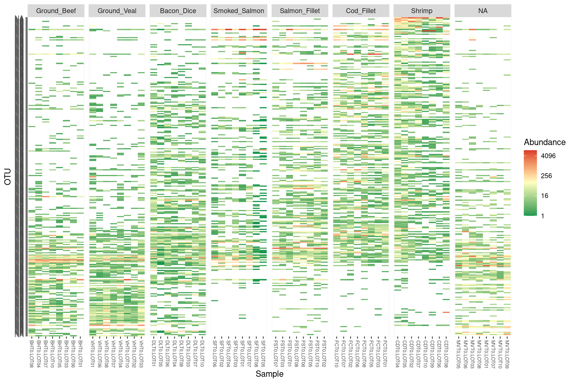
## or
## plotly::ggplotly(p)
## for an interactive version
A few conclusions
The different elements we’ve seen allow us to draw a few conclusions:
- different foods harbor different ecosystems;
- they may harbor a lot of taxa, the effective number of species is quite low;
- the high observed number of OTUs in dices of bacon is caused to by salt addition, which also moves bacon samples towards seafoods.
- the samples are really different and well separated when considering the UniFrac distance (in which case food origin accounts for 63% of the total variability)
- differential analyses is helpful to select and zoom at specific portions of the count table.